DeepWave: A Recurrent Neural-Network for Real-Time Imaging

Table of Contents

1. Introduction

2. Background

3. Proximal Gradient Descent

4. Methods

1. Introduction

Previous work: Delay-And-Sum (DAS) beamformer [1, Chapter 5]. Idea: Real-time reconstruction of acoustic spherical maps based on LISTA [2]. Limitations: It can reconstruct only high resolution microphone arrays

2. Background

2.1 Steering Matrix

The steering matrix is a matrix that contains the steering vectors of the microphone array. The steering vector is a vector that contains the phase shifts of the microphones in the array.
Signals can arrive to the microphones from different positions and angles. A direction can be parametrized as:

• Azimuth \(\theta\): The horizontal angle of arrival.
• Elevation \(\phi\): The vertical angle of arrival.

The vector that stores the phase shifts or time delays of the signal to each microphone in the array is the steering vector. The steering vector is a complex 1D vector of \( M \) elements (microphones), \( a(\theta) \in \mathbb{C}^{M} \): \[ \mathbf{a}(\theta) = \begin{pmatrix} 1 \\ e^{-j k d \sin(\theta)} \\ e^{-j 2 k d \sin(\theta)} \\ \vdots \\ e^{-j (M-1) k d \sin(\theta)} \end{pmatrix} \label{eq:steering-vector} \tag{Eq. 1} \] where:

• \( k = \frac{2 \pi}{\lambda} \) is the wavenumber.
• \( d \) is the distance between the microphones.
• \( \lambda \) is the wavelength.

When we have multiple sources or multiple angles of arrival, we can generalize the steering vector in a steering matrix. Supposing that we have different signals arriving from angles \( \theta_1, \cdots,\theta_N \), being \( N \) the number of sources, the steering matrix \( \boldsymbol{A} \in \mathbb{C}^{M \times N} \) is defined as: \[ \boldsymbol{A} = (a(\theta_1),...,a(\theta_N)) = \begin{pmatrix} 1 & 1 & \cdots & 1 \\ e^{-j k d \sin(\theta_1)} & e^{-j k d \sin(\theta_2)} & \cdots & e^{-j k d \sin(\theta_N)} \\ e^{-j 2 k d \sin(\theta_1)} & e^{-j 2 k d \sin(\theta_2)} & \cdots & e^{-j 2 k d \sin(\theta_N)} \\ \vdots & \vdots & \ddots & \vdots \\ e^{-j (M-1) k d \sin(\theta_1)} & e^{-j (M-1) k d \sin(\theta_2)} & \cdots & e^{-j (M-1) k d \sin(\theta_N)} \end{pmatrix} \label{eq:steering-matrix} \tag{Eq. 2} \]

3. Proximal Gradient Descent

DeepWave reconstructs the images with a Recurrent Neural Network trained with Proximal Gradient Descent (PGD) by optimizing: \[ \hat{x} = \arg \min_{\mathbf{x} \in \mathbb{R}^{N}_{+}} \frac{1}{2} \| \hat{\Sigma} - \mathbf{A} \, \text{diag}(\mathbf{x}) \, \mathbf{A} ^ H \|^2_F \quad + \quad \lambda \left[ \gamma \| \mathbf{x} \|_1 + (1 - \gamma) \| \mathbf{x}\|_2^2 \right], \label{eq:objective-function} \tag{Eq. 3} \] which, after vectorization becomes: \[ \hat{x} = \arg \min_{x \in \mathbb{R}^{N}_{+}} \frac{1}{2} \| \text{vec} (\hat{\Sigma}) - (\overline{\mathbf{A} } \, \circ \mathbf{A} ) \, \|^2_F \quad + \quad \lambda \left[ \gamma \| \mathbf{x}\|_1 + (1 - \gamma) \| \mathbf{x}\|_2^2 \right], \label{eq:objective-function-vectorized} \tag{Eq. 4} \] where:

• \( \hat{x} \) is variable being optimized..
• \( \hat{\Sigma} \) is the estimated covariance matrix.
• \( \boldsymbol{A} \in \mathbb{C}^{M \times N} \) is the steering matrix.
• \( \boldsymbol{A} ^ H \) is the Hermitian of the steering matrix.
• \( \text{diag}(x) \) is a diagonal matrix with the elements of \( x \).
• \( \lambda \) is the regularization parameter.
• \( \gamma \) is the regularization parameter, the trade-off parameter between the \( \ell_1 \) and \( \ell_2 \) norms.
• \( \overline{\boldsymbol{A} } \) is the conjugate of the steering matrix.
• \( \circ \) is the Hadamard product.
• \( \| \cdot \|_F \): The Frobenius norm, which measures the difference between the target matrix and the approximation.

Proximal Gradient Descend (PGD) allows to approximate the expressions above with the following: \[ \mathbf{x}^{k} = \text{ReLU} \left( \frac{\mathbf{x}^{k-1} - \alpha (\overline{\mathbf{A}} \circ \mathbf{A})^H \left[ (\mathbf{A} \circ \mathbf{A}) \mathbf{x}^{k-1} - \text{vec}\left( \hat{\Sigma} \right) \right] - \lambda \alpha \gamma}{2 \lambda \alpha (1 - \gamma) + 1}\right) \quad k \geq 1, \label{eq:proximal-gradient-descent} \tag{Eq. 5} \]

4. Methods

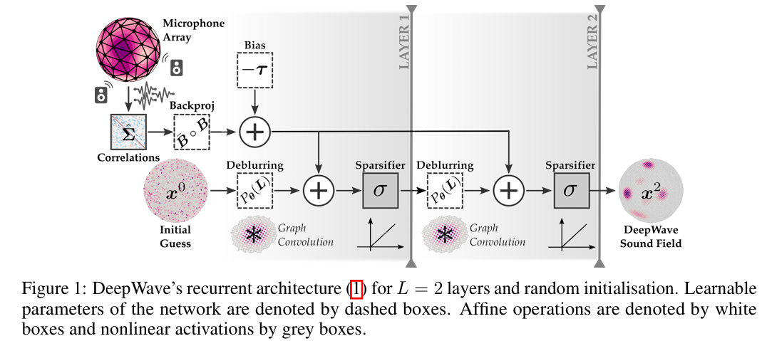
Given the covariance matrix \( \hat{\Sigma} \in \mathbb{C}^{M \times M} \), where \( M \) is the number of microphones, the network reconstructs the spherical acoustic map (SAM) with 2 layers. \( \mathbf{x} \) denotes the neuron at layer \( l \) in Eq. 6 and Fig. 1.

The trainable parameters are \( P_\theta (\mathbf{L}) \), \( \mathbf{\hat{B}} \), and \( \tau \). The network is trained with the objective function in Eq. 4. \[ \mathbf{x}^{l} = \sigma (P_\theta (\mathbf{L}) \ \mathbf{x}^{l-1} + [\mathbf{\hat{B}} \circ \mathbf{B]^H \ \mathrm{vec}} (\hat{\Sigma}) - \tau), \quad l=1,...,L \label{eq:neuron} \tag{Eq. 6} \] where:

• \( \mathbf{x}^{l} \) is the neuron at layer \( l \).
• \( \sigma \) is the ReLU activation function.
• \( P_\theta \) is the deblurring operator and \( P_\theta (\mathbf{L}) \) the deblurring matrix.
• \( \mathbf{L} \in \mathbb{R}^{N\times N} \) is the graph Laplacian.
• \( \mathbf{\hat{B}} \) is the conjugate of the steering matrix.
• \( \mathbf{B} \) is the steering matrix.
• \( \tau \) is the threshold.
• \( \hat{\Sigma} \) is the estimated covariance matrix.
• \( \mathrm{vec}(\cdot) \) is the vectorization operation.
  Let \( \mathbf{A} \in \mathbb{C}^{M \times N} \) be a matrix, where \( M \) is the number of rows and \( N \) is the number of columns. The vectorization operator \( \mathrm{vec}(\cdot) \) reshapes the matrix \( \mathbf{A} \) into a vector of dimension \( M \ N \times 1 \) by stacking its columns: \( \mathrm{vec}(A) \in \mathbb{C}^{M \ N \times 1} \). The operation is defined as: \[ [\mathrm{vec}(\mathbf{A})]{M(j-1)+i} = [\mathbf{A}]{ij} \quad \mathrm{for} \quad i = 1, \ldots, M \mathrm{ \quad and \quad } j = 1, \ldots, N \label{eq:vectorization} \tag{Eq. 7} \]

The