Paper Title
Generative modeling by estimating gradients of the data distribution
Yang Song and Stefano Ermon
In Advances in Neural Information Processing Systems (NeurIPS), 2019
score-based models, diffusion models
title={Generative modeling by estimating gradients of the data distribution},
author={Song, Yang and Ermon, Stefano},
journal={Advances in neural information processing systems},
year={2019},
volume={32},
}
TL;DR: This work establishes score-based generative modeling by connecting score matching with generative modeling across multiple noise levels. It learns the score of the log data density through a score model and leverages Langevin dynamics with annealing for high-quality sampling.
1. Introduction
This paper introduces the following concepts:
- Score-based generative modeling. It introduces a new generative approach by learning the score function \( \nabla_\mathbf{x} \log p(\mathbf{x}) \) of the data distribution at multiple noise levels. The new approach is called score-based generative modeling and it is based on the idea of estimating the gradient of the data distribution (log density) instead of learning directly the data distribution itself. This simplifies the learning process.
- Multi-level noise conditioning. Inspired by annealing processes, this work poposes to condiiton the score model on different noise scales. This allows to capture low data density regions and improve the quality of the samples.
- Connect score matching with generative modeling. This work leverages denoising score matching [Vincent 2011] by training a score network which predicts gradients of noised data densities. By iterative refinement, the model can producce high-quality samples. This is connected with the points above and, in addition to them, establishes the so-called score-based generative modeling.
- Annealed Langevin dynamics for sampling. Sampling is achieved using Langevin dynamics where noise levels are gradually reduced or annealed to guide the samples from initial random noise toward the data distribution. This process is called annealed Langevin dynamics and addresses the slow mixing issues in high-dimensional sampling. Note: Take into ccount that this paper likely established score-based generative modeling while Denoising Diffusion Probabilistic Models (DDPM) [Ho et al. 2020]. While this paper proposes advances in pure score-based models, DDPM connect score-based models and diffusion processes (that is, the forward and backward learning processes) and therefore, defined the well-known diffusion models.
2. Score Matching and Langevin Dynamics
The basic idea behind the so-called score-based generative modeling, also known as diffusion models, is to train a score network such that \( s_\theta(\mathbf{x}) \approx \nabla_x \log p_{data}(\mathbf{x}) \) and then approximately obtain samples with Langevin dynamics using the score network \( s_\theta(\mathbf{x}) \). For that, we need to estimate the gradient of the data distribution with score matching. Therefore, we will introduce Langevin dynamics in this section, and then review score matching approaches.
2.1 Score Matching
Given a large dataset, we can use principle statistical methods like score matching to train a score model to estimate the underlying score function. In order to build a genertative model, we have to find a certain approach to create new datapoints from the given vector field of score functions.

Fig. 1. Generative modeling approach.
Suppose we are given the score function \( s_\theta(\mathbf{x}) \) (Fig. 1, left) and imagine that there are many random points scattered accross it (Fig. 1, middle). Can we move those data points to form samples from the score function? One idea is that we can potentially move those points by following the directions predicted by the score function. However this will not give us valid samples because all of those points will eventually collapse into each other (Fig. 1, right).
This problem can be addressed by following a noise inversion of the score function. Equivalently, we inject gaussian noise to our score function and follow those noise perturbed score functions (Fig. 1, right). If we keep this sampling procedure long enough to reach convergence, and if we set the step size to be very very small, then this method will give us the correct samples from the score function. This method is the well-known approach of Langevin dynamics [Parisi 1981], [Grenander and Miller 1994]. Before dive in the Langevin dynamics, we will review the score matching approach.
2.2 Langevin Dynamics
Langevin dynamics describes a type of stochastic differential equation (SDE) commonly used to model the evolution of systems subject to both deterministic forces and random fluctuations (noise). In its most basic form, Langevin dynamics for a particle can be written as: \[ \frac{d\mathbf{x}}{dt} = \underbrace{-\nabla U(\mathbf{x})}_{\text{Deterministic}} + \underbrace{\gamma \mathbf{z}(t)}_{\text{Stochastic}}, \tag{Eq. 1} \label{eq:langevin-dynamics} \] where:
- \( \mathbf{x} \) is the position of the particle.
- \( U(\mathbf{x}) \) is the potential energy function.
- \( \gamma \) is the noise strength coefficient.
- \( \mathbf{z}(t) \) is the stochastic term, often Gaussian nosise.
2.1.1. Discretized Langevin Dynamics
The discretized version of Langevin dynamics, which is a variation of Euler-Maruyama method, is given by: \[ \mathbf{x}_{t} = \mathbf{x}_{t-1} + \frac{\epsilon}{2} \nabla_\mathbf{x} U(\mathbf{x}_t) + \sqrt{\epsilon} \, \mathbf{z}_t, \tag{Eq. 2} \label{eq:discretized-langevin-dynamics} \] where:
- \( \epsilon > 0 \) is the step size.
- \( \mathbf{z}_t \) is the noise term, often Gaussian noise.
- \( \mathbf{x}_0 \sim \pi(\mathbf{x}) \) is the initial value with \pi being a prior distribution.
- \( \mathbf{z}_t \sim \mathcal{N}(0,I) \).
Notice that with this formulation, we can train our score network such that \( s_\theta(\mathbf{x}) \approx \nabla_\mathbf{x} \log p_{data} \) and then obtain approximate samples from \( p_{data} \) through Langevin dynamics using the score network \( s_\theta(\mathbf{x}) \).
2.1.2. Annealed Langevin Dynamics
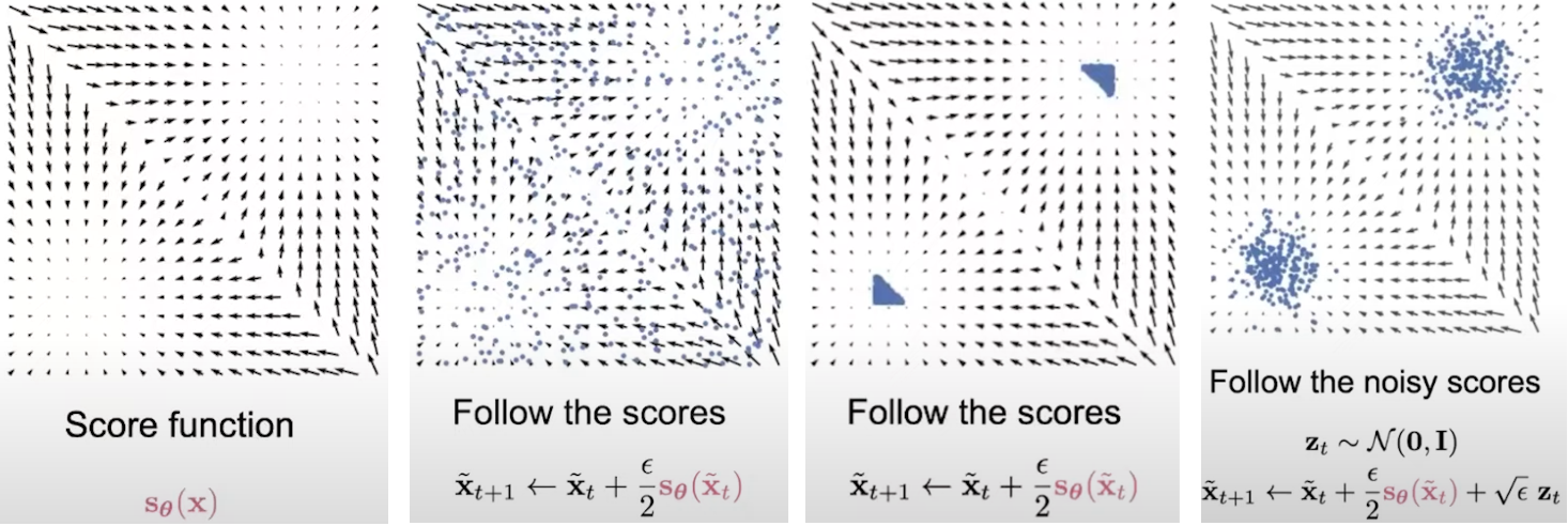
Fig. 2. Langevin dynamics for score-matching.
2.1.3. Sampling Langevin Dynamics
6: \( \tilde{\mathbf{x}}_t \leftarrow \tilde{\mathbf{x}}_{t-1} + \frac{\alpha_i}{2} s_\theta(\tilde{\mathbf{x}}_{t-1}, \sigma_i) + \sqrt{\alpha_i} \, \mathbf{z}_t \)
7: end for
2.3. Score Matching + Langevin Dynamics
Combining score matching and Langevin dynamics naively does not produce good empirical results. There are several challenges that should be addressed to make this combination work.
For example, it is hard to estimate score functions accurately in low data density regions.
Consider the density function (Fig. 3, left), the ground truth score function (Fig. 3, middle) and the estimated score function (Fig. 3, right).
If we compare the estimated and ground truth scores, we can observe how accurate are they in high density regions (green boxes).
But for low data density regions, the estimated scores are not accurate at all.
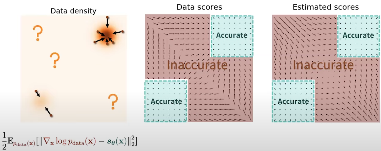
Fig. 3. Density regions scores.
How to address this challenge?
One idea is to inject Gaussian noise to perturb our data points. After adding enough Gaussian noise, we would perturb the data points to everywhere in the space. This means the size of low data density regions becomes smaller. In the image domain, this means adding Gaussian noise to perturb each pixel of the image. We can see in Fig. 4 how the estimated score now become accurate almost everywhere.
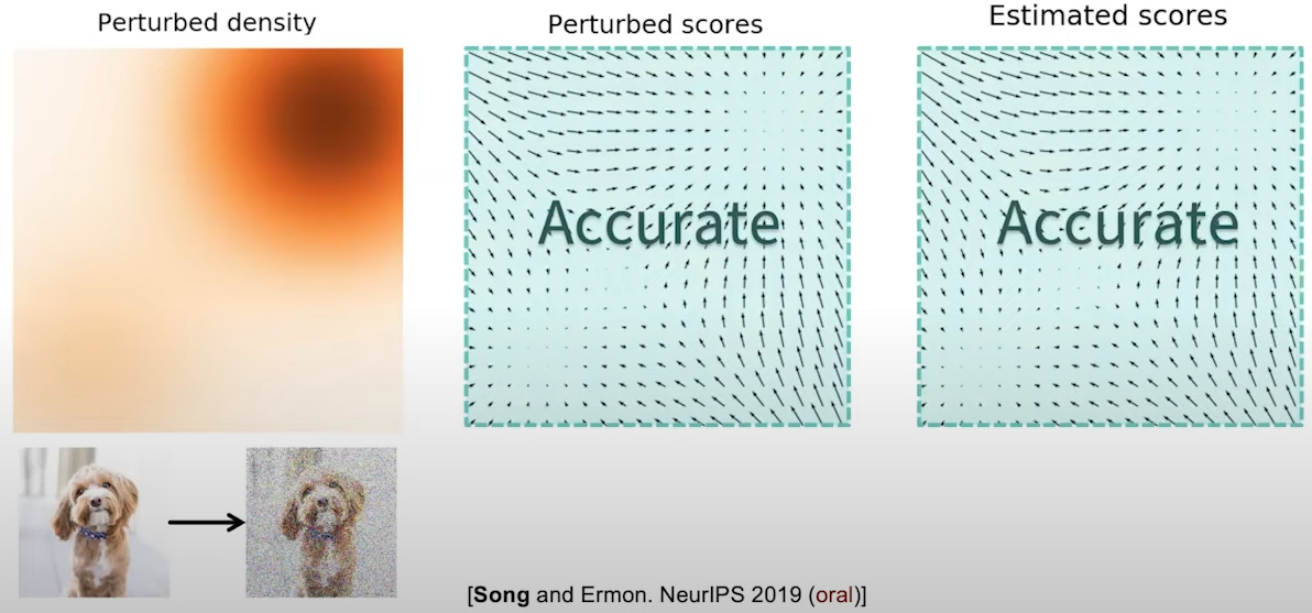
Fig. 4. Density regions scores after perturbation of data points.
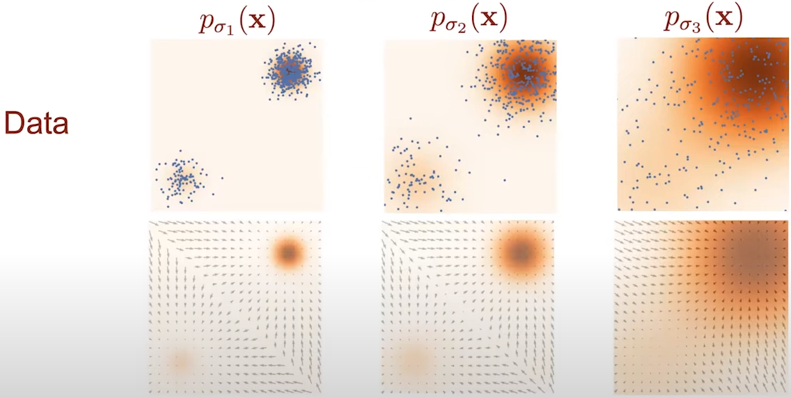
Fig. 5. Density regions across different noise levels.

Fig. 6. Image perturbation with different noise levels.
But, how can we estimate three noisy score functions?
The most naive approach is to train three neural networks so each network will estimate the score function of a single noise level. This is not a scalable solution because in practice, we might require much more noise levels. Another approach is to consider a noise conditional score model. A noise conditional score model is a simple modification of our score model which takes the noise level $\sigma$ as one additional input dimension. The output corresponds to the score function of the data density perturbed with noise level \( \sigma \).
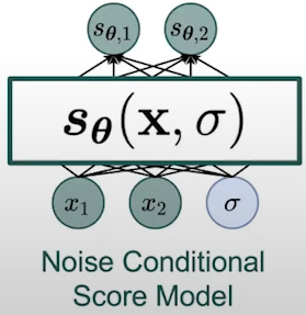
Fig. 7. Noise conditional score model.
So, how can we train this noise conditional score model?
We can leverage the idea of score matching. The score matching objective needs to be modified to jointly train the score model across all levels. In such modification, we have a summation with score matching losses. We have one socre matching loss for each noise level \( \sigma_i \) and a positive weighting function \( \lambda(\sigma_i) \). The loss is a generalization to the training objective of the first version of diffusion probabilistic models [Sohl-Dickstein et al. 2015]. It connects score-based models with diffusion models was first unveiled by the Denoising Diffusion Probabilistic Models (DDPM) [Ho et al. 2020]. The score matching loss floows the expression: \[ \frac{1}{N} \sum_{i=1}^{N} \underbrace{\lambda(\sigma_i)}_{\text{Positive weighting function}} \underbrace{\mathbb{E}_{p_{\sigma_i}(\mathbf{x})} \left[ \left\| \nabla_{\mathbf{x}} \log p_{\sigma_i}(\mathbf{x}) - s_{\theta}(\mathbf{x}, \sigma_i) \right\|_2^2 \right]}_{\text{Score matching loss}}, \tag{Eq. 3} \label{eq:score-matching-loss} \] The weighting function \( \lambda \) balances the scales of score matching loss across all noise levels, which is helpful for optimizaion. The value of the weighting function is typically chosen using people's heuristics but it can also be derive using principled analysis of the problem. By minimizing this modified score matching loss, if out optimizer is powerful enough, and our model expressive enough, then we will obtain an accurate score estimation for all noise labels.
After training this noise-conditional score model, how can we generate samples?
We can use Langevin dynamics. First, we can use Langevin dynamics to sample from the score model with the biggest perturbation of noise. the samples will be used as the initialization to sample from the score model fo the next noise level. We continue doing this process untill finally generate samples from the score function with the smallest noise level. This procedure is called **Annealed Langevin dynamics** because the rough intuition is hoping to gradually anneal down the temperature of our data density to gradually reduce the noise level. We can start from random noise, then modify the data according to the score model and the output will be accurate. This method outperform GANS (the best performing method for sample generation to that date) in inception score, but it does not in FID.