Paper Title
High-Resolution Image Synthesis with Latent Diffusion Models
Robin Rombach, Andreas Blattmann, Dominik Lorenz, Patrick Esser and Björn Ommer
In Conference on Computer Vision and Pattern Recognition (CVPR), 2023
diffusion models, latent diffusion, VQ-VAE
@inproceedings{Rombach2022latent,
title={High-Resolution Image Synthesis with Latent Diffusion Models},
author={Robin Rombach andAndreas Blattmann and Dominik Lorenz and Patrick Esser and Bj{\"{o}}rn Ommer},
booktitle={{IEEE/CVF} Conference on Computer Vision and Pattern Recognition, {CVPR}}
year={2023},
pages={10674--10685},
publisher={{IEEE}},
}
title={High-Resolution Image Synthesis with Latent Diffusion Models},
author={Robin Rombach andAndreas Blattmann and Dominik Lorenz and Patrick Esser and Bj{\"{o}}rn Ommer},
booktitle={{IEEE/CVF} Conference on Computer Vision and Pattern Recognition, {CVPR}}
year={2023},
pages={10674--10685},
publisher={{IEEE}},
}
TL;DR: Introduced Latent Diffusion Models that operate in a lower-dimensional latent space rather than the pixel space. This innovation reduced computational costs and enabled diffusion models to handle higher-resolution images and complex tasks like text-to-image generation.
2. Model
2.1 Neural Network (Denoiser): Autoencoder
Diffusion models [Shohl-Dickstein et al. 2015] are a class of generative models that operate in the pixel space. They model the data distribution by iteratively applying a series of noise levels sampled from a predefined distribution to the input image, governed by a stochastic time-dependent process that dictates the transition of data distributions over time (Fig. 1).
However, pixel space is a high-dimensional space which makes them computationally expensive, specially during the reverse diffusion process or denoising.
This paper uses an Autoencoder, specially, a VQ-VAE to convert the pixel space into a latent space and therefore, reduce the computational complexity of the denoising process. Also, the latent space is powerful for conditional sampling.
An autoencoder is composed by an Encoder \( \mathcal{E} \) and a Decoder \( \mathcal{D} \). The encoder maps the input image \( x \) to a lower-dimensional latent space \( z \). The decoder maps the latent space \( z \) to the output image \( x \).
This paper uses a VQ-VAE in the middle of the diffusion process, which is basically using the VQ-VAE to denoise or, in other words, to predict the noise level of the input image at each time step of the reverse diffusion process.
In particular, the Autoencoder is a UNet-based VQ-VAE that predicts the noise level of the input image \( x_t \) that we want to remove. The input of the Unet is a noisy image which contains the noise-level correspondint to step time \( t \).
This way, we input an image in the pixel space and generate a latent space representation of it.
One of the core contributions of this paper is to use the latent space of the VQ-VAE for conditional sampling.
2.2 Training
Then, we can summarize the training process in 2 steps: training the autoencoder and training the diffusion process in the latent space. These steps are trained separately.
2.2.1 Autoencoder Training
A vanilla autoencoder is trained with an input \( \mathbf{x} \) and it predicts the same image \( \mathbf{\hat{x}} \).
In this paper, to train the VQ-VAE along with the diffusion process which depends on time \( t \), the authors train the model in an adversarial manner.
A discrimiator decoder \( \mathcal{D}_\phi \) is used to discriminate the input images \( \mathbf{x} \) from the reconstructions \( \mathbf{\hat{x}} = \mathcal{D}(\mathcal{E}(\mathbf{x}))\).
The autoencoder is trained with the following loss function:
\[
\mathcal{L}_{\text{Autoencoder}} = \min_{\mathcal{E}, D} \max_{\psi} \left( \mathcal{L}_{\text{rec}}(x, D(\mathcal{E}(x))) - \mathcal{L}_{\text{adv}}(D(\mathcal{E}(x))) + \log D_{\psi}(x) + \mathcal{L}_{\text{reg}}(x; \mathcal{E}, D) \right),
\tag{Eq. 1} \label{eq:1}
\]
where:
- \( \mathcal{L}_{\text{rec}}(\mathbf{x}, \mathcal{D}(\mathcal{E}(\mathbf{x}))) = \text{MSE}(\mathbf{x}, \mathcal{D}(\mathcal{E}(\mathbf{x})))\) is the reconstruction loss, which is the mean squared error between the input image and the reconstruction. It mathches the input and predicted image by the autoencoder.
- \( \mathcal{L}_{\text{reg}}(\mathbf{x};\mathcal{E},\mathcal{D}) = \text{KL}(\mathcal{E}(\mathbf{x}, \mathcal{N}(0,1))) \) is the regularization loss, which is the commitment loss of the VQ-VAE. In short, it minimizes the difference between the latents and a normal distribution. This loss, in addition to the reconstruction loss form the vanilla VAE loss.
- \( \mathcal{L}_{\text{adv}}(\mathcal{D}(\mathcal{E}(\mathbf{x}))) = - \log D_{\psi}(\mathcal{D}(\mathcal{E}(\mathbf{x})) \approx - \log D_{\psi}(\mathbf{x}) \) is the adversarial loss, which is the log probability of the discriminator decoder \( \mathcal{D}_\phi \) which classifies the input image as real or fake. So, the total adversarial loss has the form: \[ \min_{\mathcal{E}, D} \max_{\psi} \left( -\log [\mathcal{D}_\psi(\mathcal{D}(\mathcal{E}(\mathbf{x}))] + \log D_{\psi}(\mathcal{D}(\mathbf{x}))) \right). \] This is done because we want the autoencoder to reconstruct images as good as possible plus generate real images (and not fake ones).
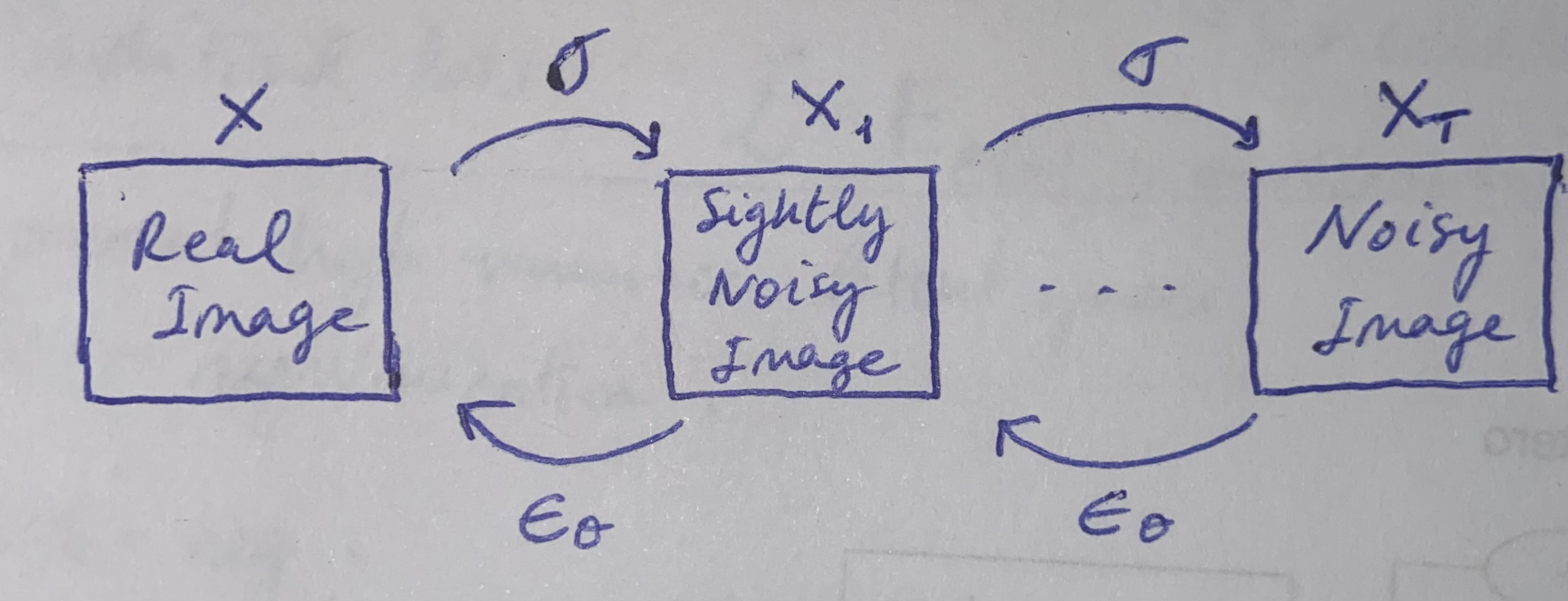
Fig. 1. Standard diffusion process.
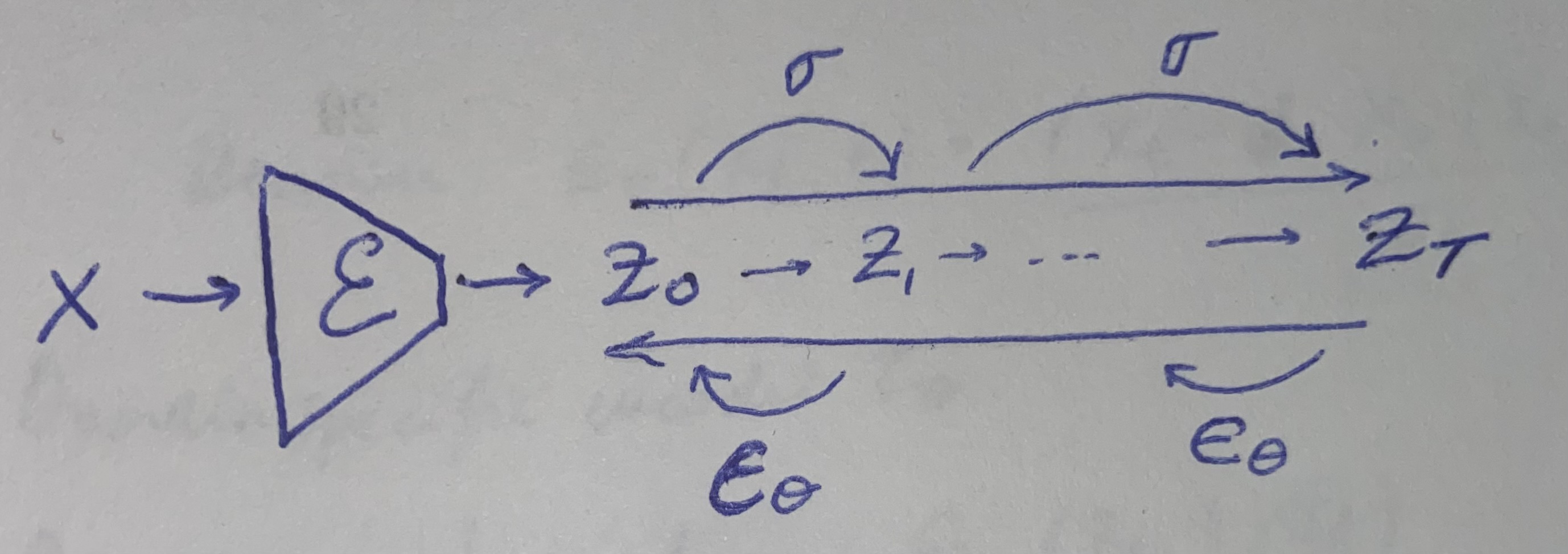
Fig. 2. Diffusion process in the latent space.
2.2.2 Diffusion Training
During the diffusion training process, the encoder and decoder are frozen.
2.3 Conditioning Sampling
Now that we trained our model,
Comments
Comments are powered by Giscus and stored as GitHub Discussions. You need a GitHub account to comment or react.
© Copyright © All rights reserved | Carlos Hernández Oliván | Colorlib